对抗攻击 (adversarial
attack)是一种针对机器学习模型的测试阶段攻击 。对抗攻击一般通过向干净测试样本对抗样本 (adversarial
example)隐蔽性 ,即让添加的噪声不易被人眼察觉,其通常会通过扰动约束 将对抗样本扰动上限 (也称扰动半径)。
image-20250817233941825
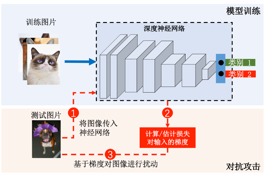
对抗攻击扰动的样本是测试样本
对抗攻击改变的是输入样本,而模型训练改变的是模型参数。所以对抗攻击需要计算(白盒攻击)或者估计(黑盒攻击)模型损失相对输入的梯度信息
对抗攻击通过梯度上升最大化模型的错误
分类:
按攻击目标分类:非目标攻击、目标攻击
按获得的先验信息分类:白盒攻击、黑盒攻击
白盒攻击
提出:
2013年,Biggio等人首次发现了攻击者可以恶意操纵测试样本 来躲避支持向量自动机和浅层神经网络的检测 ,这种攻击被称为躲避攻击(evasion
attack)。同时,Szegedy等人针对深度神经网络提出了类似的攻击并将其定义为对抗样本 (adversarial
example)。
边界约束优化问题(bound
constrained optimization problem)
其中,
由于上述优化问题难以精确求解,所以Szegedy等人转而使用边界约束的L-BFGS (Limited-memory
Broyden–Fletcher–Goldfarb–Shanno)算法(内存受限的拟牛顿法)来近似求解:
通过L-BFGS攻击方法生成的对抗样本不但能攻击目标模型,还可以在不同模型和数据集之前迁移 ,即基于目标模型生成的对抗样本也可以攻击(虽然成功率会下降)使用不同超参数或者在不同子集上训练的模型。
但是效率太低,需要对每个样本求解上述表达式
快速梯度符号方法(fast
gradient sign method, FGSM)
FGSM假设,损失函数
基于此,FGSM利用输入梯度(分类损失相对输入的梯度)的符号信息(即梯度方向 )进行一步固定步长的梯度上升 来完成攻击:
但是,FGSM攻击成功率比较低,但是简单高效啊
1
2
3
4
5
6
7
8
9
10
11
12
13
14
15
16
17
18
19
20
21
def fgsm_untargeted_attack (image_tensor, epsilon, data_grad ): """ 执行非目标性FGSM的核心计算逻辑。 (Executes the core logic of an untargeted FGSM) :param image_tensor: 原始图片张量 (The original image tensor) :param epsilon: 扰动大小 (步长) (The perturbation magnitude) :param data_grad: 损失函数对于输入图片的梯度 (The gradient of the loss w.r.t. the input image) :return: 经过扰动处理后的新图片张量 (The new perturbed image tensor) """ gradient_sign = data_grad.sign() perturbed_tensor = image_tensor + epsilon * gradient_sign perturbed_tensor = torch.clamp(perturbed_tensor, 0 , 1 ) return perturbed_tensor
基于FGSM提出的基本迭代攻击方法(basic
iterative method,BIM)
因为L-BFGS,FGSM都是直接将对抗样本输入到深度神经网络模型中
为了对抗样本更好地应用于物理世界,提出了BIM
BIM以更小的步长多次应用FGSM ,并在每次迭代后对生成的对抗样本的像素值进行裁剪 ,以保证每个像素的变化都足够小
每次在上一步的对抗样本的基础上,各个像素增长$ ( 或 者 减 少 ) , 然 后 再 执 行 裁 剪 , 保 证 新 样 本 的 各 个 像 素 都 在 的
1
2
3
4
5
6
7
8
9
10
11
12
13
14
15
16
17
18
19
20
21
22
23
24
25
26
27
28
29
30
31
32
33
34
35
36
37
38
39
40
41
42
def bim_untargeted_attack (model, original_image_tensor, epsilon, alpha, num_iterations, device ): """ 执行非目标性BIM攻击的核心计算逻辑。 (Executes the core logic of an untargeted BIM) :param model: 目标模型 (The target model) :param original_image_tensor: 原始图片张量 (The original image tensor) :param epsilon: 允许的最大扰动 (L-infinity norm) (Maximum perturbation allowed) :param alpha: 每步的步长 (Step size for each iteration) :param num_iterations: 迭代次数 (Number of iterations) :param device: 计算设备 (cpu or cuda) (Computation device) :return: 经过扰动处理后的新图片张量 (The new perturbed image tensor) """ perturbed_image = original_image_tensor.clone().detach() original_label = torch.tensor([0 ], device=device) criterion = nn.CrossEntropyLoss() for i in range (num_iterations): perturbed_image.requires_grad = True output = model(perturbed_image) loss = criterion(output, original_label) model.zero_grad() loss.backward() adv_temp = perturbed_image.detach() + alpha * perturbed_image.grad.sign() eta = torch.clamp(adv_temp - original_image_tensor, min =-epsilon, max =epsilon) perturbed_image = original_image_tensor + eta perturbed_image = torch.clamp(perturbed_image, min =0 , max =1 ) return perturbed_image
投影梯度下降(projected
gradient descent,PGD)
有人认为,BIM本质上是对负损失函数的投影梯度下降,并提出了更加强大的迭代FGSM攻击方法—-PGD
投影 (Projection):强制 将上一步得到的结果 x为中心、半径为ε的α
迈得有多大,Proj操作都会把它拉回来,确保新的
所以,PGD的步长 α 不必像BIM那样被小心翼翼地设置为
ε/T 这种小值来间接控制扰动范围
PGD攻击被广泛认为是最强的一阶攻击方法 ,因为从非凸约束优化问题的角度来讲,PGD算法是其最好的一阶求解器。
1
2
3
4
5
6
7
8
9
10
11
12
13
14
15
16
17
18
19
20
21
22
23
24
25
26
27
28
29
30
31
32
33
34
35
36
37
38
39
40
41
42
43
44
45
46
def pgd_attack (model, original_image_tensor, epsilon, alpha, num_iterations, device ): """ 执行PGD目标性攻击 (Execute a targeted PGD attack)。 :param model: 目标模型 (The target model)。 :param original_image_tensor: 原始图片的Tensor (Tensor of the original image)。 :param epsilon: 允许的最大扰动 (L-infinity norm) (Maximum perturbation allowed)。 :param alpha: 每步的步长 (Step size for each iteration)。 :param num_iterations: 迭代次数 (Number of iterations)。 :param device: 计算设备 (cpu or cuda) (Computation device)。 :return: 扰动后的图片Tensor (The perturbed image Tensor)。 """ target = torch.tensor([1 ], device=device) criterion = nn.CrossEntropyLoss() perturbed_image = original_image_tensor.clone().detach() for i in range (num_iterations): perturbed_image.requires_grad = True output = model(perturbed_image) loss = criterion(output, target) model.zero_grad() loss.backward() perturbed_image = perturbed_image.detach() - alpha * perturbed_image.grad.sign() eta = torch.clamp(perturbed_image - original_image_tensor, -epsilon, epsilon) perturbed_image = torch.clamp(original_image_tensor + eta, 0 , 1 ) return perturbed_image
动量迭代快速梯度符号方法(momentum
iterative FGSM,MI-FGSM)
虽然BIM比FGSM攻击性更强,但其在每次迭代时都沿梯度方向“贪婪地”移动对抗样本,容易使对抗样本陷入糟糕的局部最优解 ,并过拟合于当前模型。这导致其生成的对抗样本的跨模型迁移性较差
Dong等人将动量 结合到BIM算法中,获得稳定的扰动方向 并帮助对抗样本在迭代中摆脱局部最优解
1
2
3
4
5
6
7
8
9
10
11
12
13
14
15
16
17
18
19
20
21
22
23
24
25
26
27
28
29
30
31
32
33
34
35
36
37
38
39
40
41
42
43
44
45
46
47
48
49
50
51
52
53
54
55
56
57
58
def mi_fgsm_untargeted_attack (model, original_image_tensor, epsilon, alpha, num_iterations, decay_factor, device ): """ 执行非目标性MI-FGSM攻击的核心计算逻辑。 (Executes the core logic of an untargeted MI-FGSM) :param model: 目标模型 :param original_image_tensor: 原始图片张量 :param epsilon: 允许的最大扰动 :param alpha: 每步的步长 :param num_iterations: 迭代次数 :param decay_factor: 动量衰减因子 mu :param device: 计算设备 :return: 经过扰动处理后的新图片张量 """ perturbed_image = original_image_tensor.clone().detach() momentum = torch.zeros_like(original_image_tensor, device=device) original_label = torch.tensor([0 ], device=device) criterion = nn.CrossEntropyLoss() for i in range (num_iterations): perturbed_image.requires_grad = True output = model(perturbed_image) loss = criterion(output, original_label) model.zero_grad() loss.backward() grad = perturbed_image.grad.data grad_norm_l1 = torch.norm(grad, p=1 ) if grad_norm_l1 == 0 : normalized_grad = grad else : normalized_grad = grad / grad_norm_l1 momentum = decay_factor * momentum + normalized_grad adv_temp = perturbed_image.detach() + alpha * momentum.sign() eta = torch.clamp(adv_temp - original_image_tensor, min =-epsilon, max =epsilon) perturbed_image = original_image_tensor + eta perturbed_image = torch.clamp(perturbed_image, min =0 , max =1 ) return perturbed_image
基于雅可比显著性图的攻击(Jacobian-based
saliency map attack, JSMA)
大多数攻击都是对整个样本(比如整张图片)进行扰动,同时通过限制对抗噪声的
JSMA进行更稀疏的对抗攻击(如只改变几个像素),是一种限制对抗噪声的
JSMA是一种贪心算法,每次迭代时挑选一个像素进行修改。
首先:计算模型的对抗梯度(雅可比矩阵):
接着,JSMA使用对抗梯度计算一个显著性图:
(该图包含每个像素对分类结果的影响大小 :越大的值表明修改它将显著增加被分类为目标类别的概率)
在显著性图中,每个像素
给定显著性图,JSMA每次选择一个最重要的像素 并修改它以增加目标类别的概率。重复这一过程,直到超过预先设定的像素修改个数或者攻击成功。
缺点就是,计算对抗梯度成本较大,JSMA运行速度极慢。(太tm慢了。。。)
1 2 3 4 5 6 7 8 9 10 11 12 13 14 15 16 17 18 19 20 21 22 23 24 25 26 27 28 29 30 31 32 33 34 35 36 37 38 39 40 41 42 43 44 45 46 47 48 49 50 51 52 53 54 55 56 57 58 59 60 61 62 63 64 65 66 THETA = 2.0 / 255.0 MAX_PERTURBATION_PERCENT = 0.9 def compute_jacobian (model, image_tensor, device ): """计算模型输出关于输入的雅可比矩阵""" image_tensor_clone = image_tensor.clone().detach().requires_grad_(True ) output = model(image_tensor_clone) num_features = int (np.prod(image_tensor_clone.shape[1 :])) jacobian = torch.zeros(output.size(1 ), num_features, device=device) for i in range (output.size(1 )): model.zero_grad() output[:, i].backward(retain_graph=True ) jacobian[i] = image_tensor_clone.grad.view(-1 ) return output, jacobian def jsma_targeted_attack (model, original_image_tensor, theta, max_perturb_percent, device ): """ 执行一次完整的、目标性的JSMA攻击。 """ perturbed_image = original_image_tensor.clone().detach() target_class = 1 num_pixels = torch.numel(perturbed_image) max_pixels_to_change = int (max_perturb_percent * num_pixels) search_space = torch.ones(num_pixels).to(device) for i in range (max_pixels_to_change): if (i + 1 ) % 100 == 0 : print (f" - JSMA 内部迭代 {i + 1 } /{max_pixels_to_change} ..." ) output, jacobian = compute_jacobian(model, perturbed_image, device) current_prediction = torch.argmax(output, dim=1 ).item() if current_prediction == target_class: print (f" - 在修改了 {i} 个像素后攻击成功!" ) return perturbed_image target_grad = jacobian[target_class] other_grads = jacobian.sum (dim=0 ) - target_grad mask1 = (target_grad > 0 ) mask2 = (other_grads < 0 ) mask = mask1 & mask2 & (search_space > 0 ) saliency_scores = -target_grad * other_grads * mask.float () if torch.sum (saliency_scores) == 0 : print (" - 找不到有效的像素进行修改,本次攻击尝试终止。" ) return perturbed_image best_pixel_idx = torch.argmax(saliency_scores) search_space[best_pixel_idx] = 0 pixel_indices = np.unravel_index(best_pixel_idx.cpu().numpy(), perturbed_image.shape) perturbed_image[pixel_indices] += theta perturbed_image = torch.clamp(perturbed_image, min =0 , max =1 ) return perturbed_image
基于优化的CW攻击(Carlini-Wagner)攻击算法
直接将噪声大小直接放到优化目标里进行最小化优化,具体是求解下述问题:
与L-BFGS攻击方法不同,CW攻击引入了一个新的变量
CW攻击有三个版本: 它衡量的是被修改过的像素个数。只修改图中极少数几个像素 ,但被修改的像素颜色值可能会有比较大的变化
确定一些对模型输出影响不大的像素 ,然后固定这些像素值不变,直到修改剩下的像素也无法再生成对抗样本。而像素的重要性是由
它衡量的是噪声的“整体能量”。会给图片的很多像素 都加上一点点微弱的改动
它衡量的是所有被修改像素中改动最大的那一个。可以有很多像素被修改,但没有一个像素改动得特别突出
由于
每次迭代后,如果对于所有的
CW攻击可以被认为是最强的单体白盒攻击 方法(PGD只是一阶最强)。CW攻击算法攻破了许多曾被认为是有效的防御策略,然而其生成对抗样本的计算开销很大。
1 2 3 4 5 6 7 8 9 10 11 12 13 14 15 16 17 18 19 20 21 22 23 24 25 26 27 28 29 30 31 32 33 34 35 36 37 38 39 40 41 42 43 44 45 46 47 48 49 50 51 52 53 54 55 56 57 58 59 60 61 62 63 64 65 66 67 68 69 70 71 72 73 74 75 76 77 78 79 80 81 82 83 CONFIDENCE = 0 LEARNING_RATE = 0.01 MAX_ITERATIONS = 1000 C_SEARCH_STEPS = 10 INITIAL_C = 0.01 def cw_l2_targeted_attack (model, original_image_tensor, c_constant, confidence, learning_rate, num_iterations, device ): """ 执行目标性C&W L2攻击的核心计算逻辑。 (Executes the core logic of a targeted C&W L2) """ target_class = 1 num_classes = 2 w = torch.arctanh(2 * original_image_tensor - 1 ).clone().detach().requires_grad_(True ) optimizer = torch.optim.Adam([w], lr=learning_rate) for i in range (num_iterations): perturbed_image = 0.5 * (torch.tanh(w) + 1 ) output = model(perturbed_image) l2_loss = torch.sum ((perturbed_image - original_image_tensor) ** 2 ) target_logits = output[0 , target_class] mask = torch.ones_like(output).bool () mask[0 , target_class] = 0 other_logits = output[mask].view(1 , -1 ) max_other_logits = torch.max (other_logits) attack_loss = torch.max (max_other_logits - target_logits + confidence, torch.tensor(0.0 ).to(device)) total_loss = l2_loss + c_constant * attack_loss optimizer.zero_grad() total_loss.backward() optimizer.step() if (i + 1 ) % 100 == 0 : pred_idx = torch.argmax(output).item() print ( f" - C&W 内部迭代 {i + 1 } /{num_iterations} : Loss={total_loss.item():.4 f} , Prediction={['Duck' , 'Rabbit' ][pred_idx]} " ) final_perturbed_image = 0.5 * (torch.tanh(w) + 1 ).detach() return final_perturbed_image def main (): for i in range (C_SEARCH_STEPS): print (f"\n[第 {i + 1 } /{C_SEARCH_STEPS} 次攻击尝试] 平衡常数 C = {current_c:.4 f} " ) ..... perturbed_tensor_224 = cw_l2_targeted_attack( model, image_tensor_224, current_c, CONFIDENCE, LEARNING_RATE, MAX_ITERATIONS, device ) ...... current_c *= 10
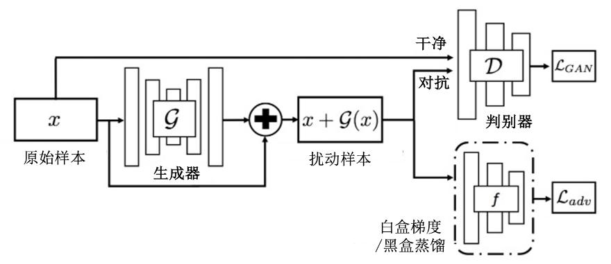
AdvGAN攻击方法
AdvGAN攻击方法:利用生成对抗网络提前学习对抗噪声的分布,之后给定任意一个干净样本都可以直接输出其所需要的对抗噪声。
image-20250818004811054
如图所示,实现针对目标模型 ,添加噪声的样本在有目标攻击中 ,损失鼓励 添加噪声的样本它可以对任何给定的输入样本产生扰动却不需要访问目标模型 。
除此之外,AdvGAN方法还可以被用于黑盒攻击,通过查询目标模型的输出来动态地训练蒸馏模型。在攻击对抗训练、集成对抗训练或PGD对抗训练的模型时,AdvGAN取得了比FGSM和CW方法更高的成功率。